AI Technical Writer

Introduction
Everyone wants to talk about training. The GPU clusters, the trillion-token datasets, the months-long runs that cost millions of dollars. But here’s the thing: once a model is trained, it needs to run. Millions of times a day. For real users. With real latency expectations and real infrastructure budgets.
That’s inference. And inference is quietly where most of the engineering work actually happens. When a user types a message into a chatbot and expects a response in under a second, the model doesn’t get to take its time. It needs to generate tokens fast, use memory efficiently, and do it at a cost that doesn’t make your cloud bill go sky high. A 70-billion-parameter model sitting on a server isn’t just a math problem, but it’s an operational one. This is where inference optimization comes in.
Over the last few years, we have been introduced to a lot of techniques to make large language models faster, leaner, and cheaper to run, without significantly losing the accuracy. Some of these techniques work at the model level, changing how weights are stored or how the network is structured. Others work at the serving level, changing how requests are batched and how memory is managed. The best deployments make use of several of them together.
In this two-part article, we will cover five of the most important techniques for LLM inference optimization:
Quantization reduces the numerical precision of model weights by shrinking a model that once needed 32 bits per number down to 8, 4, or even fewer, with surprisingly little quality loss.
Pruning removes parts of the model that aren’t pulling their weight, repetitive attention heads, dispensable layers, and near-zero-parameter layers, so the model stays capable while becoming structurally smaller.
Knowledge Distillation takes the intelligence locked inside a massive model and transfers it into a much smaller one, training the small model to think like the big one rather than learning from scratch.
KV Caching solves one of the most expensive hidden costs in autoregressive generation: the fact that every new token needs information from every previous token, by storing and reusing the intermediate computations so you don’t recalculate them over and over.
Speculative Decoding attacks the fundamental bottleneck of token-by-token generation by using a small, fast draft model to guess ahead, then having the large model verify multiple tokens at once in parallel, legally cheating the sequential nature of language generation.
Each of these techniques solves a different problem. Quantization and pruning shrink the model. Distillation replaces it with something smaller. KV caching makes memory management smarter. Speculative decoding makes generation itself faster. Together, they form a stack, and understanding how they interact is just as important as understanding each one individually.
In this two-part series, we will explore all of these inference optimization techniques in detail. In the first part, we will take a deep dive into quantization and pruning, understanding how these techniques help make large models smaller, faster, and more efficient for real-world deployment.
One thing to keep in mind as you read: these aren’t theoretical research ideas sitting in papers. They’re running in production right now. By the end of this article, you’ll understand not just what each technique does, but why it works, where it breaks down, and how to think about combining them for your own deployment scenarios. Whether you’re running a single GPU on a budget or orchestrating a multi-node H100 cluster, the same principles apply; only the knobs change.
Key Takeaways
- Quantization reduces the precision of model weights, making LLMs smaller, faster, and cheaper to run without heavily affecting quality.
- Pruning removes less important weights or connections from a model to improve efficiency and reduce memory usage.
- Techniques like GPTQ, AWQ, and LLM.int8() allow quantization of pretrained models without full retraining.
- Combining pruning and quantization can significantly optimize performance, especially for edge devices and budget-friendly deployments.
- Moderate optimization usually keeps model quality close to the original, but aggressive compression can reduce accuracy and reasoning ability.
- Calibration datasets help quantization methods understand how the model behaves in real workloads and usually require only a small amount of sample data.
- Optimization is becoming essential as organizations look for ways to deploy large models efficiently without relying on expensive GPU infrastructure.
Quantization — Shrinking the Numbers Without Losing the Meaning
Quantization is a technique used to make AI models smaller, faster, and cheaper to run by reducing the precision of the model weights and activations. Everyone wants to talk about training. But here’s the thing: does a neural network really need 32 bits to store a number? The answer, almost always, is no. And that lays the foundation of quantization. Let us start by understanding a little bit about weight and floating-point numbers.
What Is a Weight, Really?
A neural network learns data or any patterns by adjusting millions or even billions of tiny numerical values, which are called weights. These are basically the model’s “memory” or “knowledge.” During training, the model continuously updates these weights so that its predictions become more accurate.
Now the next question becomes:
How are these weights stored inside the computer? Most AI models store weights as floating-point numbers. A floating-point number is simply a way to represent numbers with decimals, such as:
0.245
-1.732
3.14159
Computers store these numbers using bits. The most common format in deep learning is:
| Format | Size |
|---|---|
| FP32 (Float32) | 32 bits |
| FP16 (Float16) | 16 bits |
| BF16 (BFloat16) | 16 bits |
| INT8 | 8 bits |
The Problem With FP32 is FP32 is accurate, but expensive.
Using 32 bits for every weight means:
- more memory usage
- slower data transfer
- higher power consumption
- expensive inference
And this leads to an important realization: Many neural networks do not actually need extremely precise numbers.
For example:
0.123456789
can often be approximated as:
0.12
without noticeably affecting the model’s output.
That idea leads directly to quantization.
Quantization is one of the most important optimization techniques in modern AI systems. The basic idea is simple: instead of storing and processing model weights using large, high-precision numbers like FP32, we convert them into smaller and more efficient formats such as FP16, BF16, INT8, or even INT4. The goal is to reduce memory usage and increase inference speed without significantly affecting the quality of the model’s output.
Large language models contain billions of parameters, and every parameter is represented as a number. In FP32 format, each parameter takes 32 bits of memory. A model with 7 billion parameters, therefore, requires massive amounts of VRAM just to load the weights. Quantization reduces the size of these numbers, allowing the same model to run on smaller GPUs, consumer hardware, edge devices, and large-scale inference servers more efficiently.
For example, a 7 billion model stored in FP32 may require around:
7 x 109 x 4 bytes = 28 GB 7 x 109 x 1 byte = 7 GB
When quantized to INT8, the same model may use roughly one-fourth of that memory. This reduction dramatically lowers infrastructure costs and improves scalability.
At the core of quantization is the idea that neural networks do not always need extremely precise decimal values to function well. During training, a model may learn weights such as:
0.18273642
But during inference, the model can often work with approximate representations of these values without noticeable quality loss. Quantization converts these floating-point numbers into lower-precision formats while preserving the overall meaning and behavior of the model.
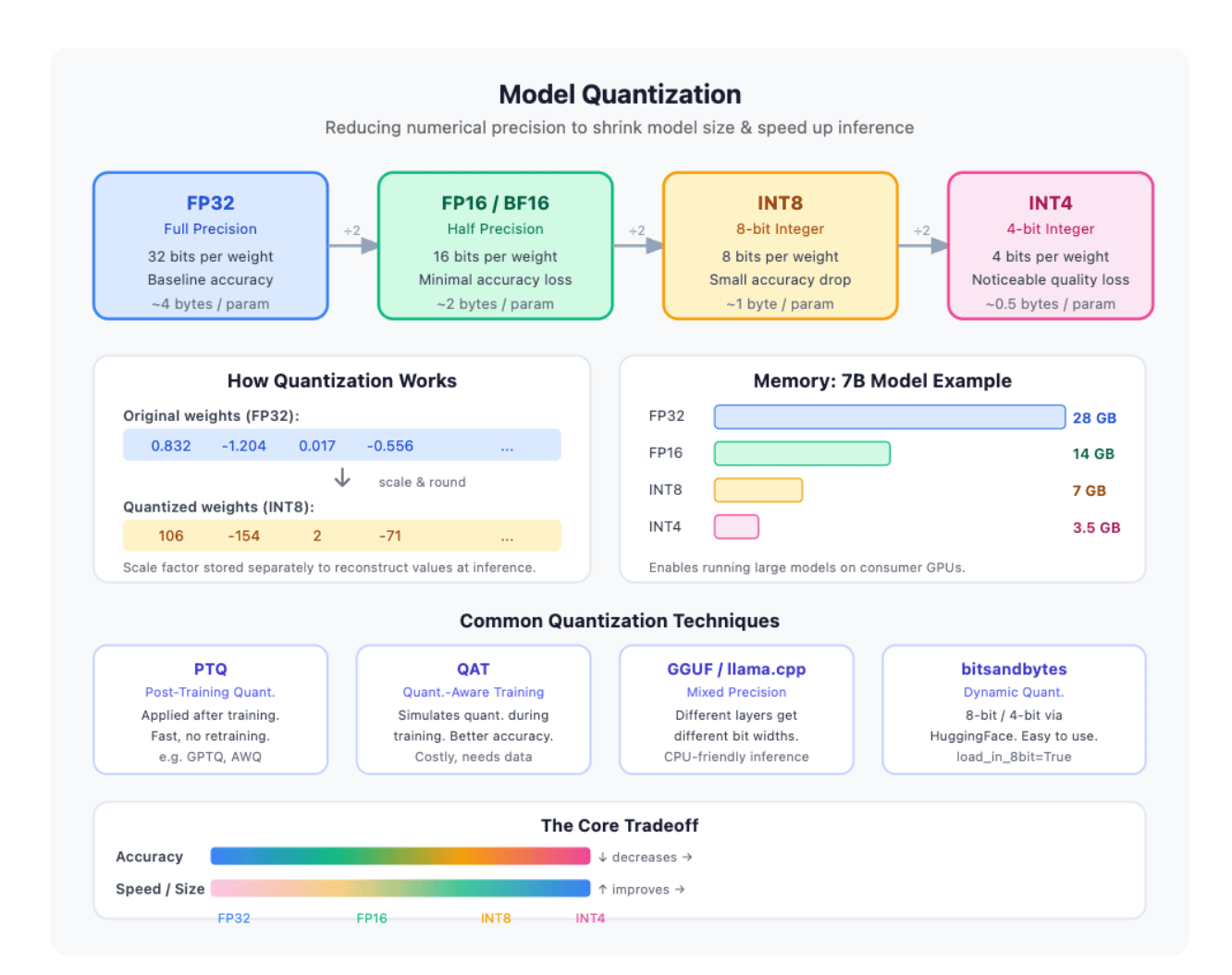
One of the most common approaches is Post-Training Quantization (PTQ). In PTQ, the model is first trained normally using FP32 or BF16 precision. After training is complete, the weights are compressed into formats like INT8 or INT4. No retraining is required, which makes PTQ fast, inexpensive, and practical for real-world deployment. This is heavily used in inference systems where the primary goal is to reduce latency and memory consumption.
PTQ example in PyTorch
import torch
import torch.nn as nn
import torch.quantization

# Simple neural network
class SimpleModel(nn.Module):
    def __init__(self):
        super(SimpleModel, self).__init__()

        self.fc1 = nn.Linear(10, 32)
        self.relu = nn.ReLU()
        self.fc2 = nn.Linear(32, 2)

    def forward(self, x):
        x = self.fc1(x)
        x = self.relu(x)
        x = self.fc2(x)
        return x


# Create model
model = SimpleModel()

# Set model to evaluation mode
model.eval()

# Specify quantization configuration
model.qconfig = torch.quantization.get_default_qconfig("fbgemm")

# Prepare the model for static quantization
torch.quantization.prepare(model, inplace=True)

# Calibration step
# Run some sample data through the model
sample_input = torch.randn(100, 10)

with torch.no_grad():
    model(sample_input)

# Convert model to INT8 quantized version
torch.quantization.convert(model, inplace=True)

# Test inference
test_input = torch.randn(1, 10)

with torch.no_grad():
    output = model(test_input)

print(output)
Another widely used technique is Dynamic Quantization, where weights are quantized ahead of time, but activations are quantized dynamically during runtime. This approach is simple to implement and works particularly well on CPUs. Frameworks like PyTorch support dynamic quantization with just a few lines of code, making it a common choice for production APIs and lightweight deployments.
quantized_model = torch.quantization.quantize_dynamic(
    model,
    {nn.Linear},
    dtype=torch.qint8
)
Static Quantization goes a step further by quantizing both weights and activations before inference begins. This requires a calibration dataset that helps determine the range of activation values the model will encounter during real usage. Because the quantization parameters are computed beforehand, static quantization often provides better performance and lower latency than dynamic quantization. It is frequently used in mobile AI systems, embedded devices, and optimized inference engines.
For scenarios where maintaining model accuracy is critical, organizations use Quantization-Aware Training (QAT). In QAT, the model simulates quantization effects during training itself. The network learns to adapt to lower precision representations while still optimizing its weights. This approach generally preserves accuracy much better than post-training quantization, especially when targeting aggressive formats like INT4. Although QAT is more computationally expensive, it is widely used in high-performance production environments where accuracy degradation is unacceptable.
Modern LLM serving systems increasingly rely on advanced quantization techniques such as GPTQ, AWQ, and GGUF formats. GPTQ, or Generalized Post-Training Quantization, focuses on reducing quantization error layer by layer, enabling large models to run efficiently in 4-bit precision with minimal quality loss. AWQ, or Activation-Aware Weight Quantization, improves upon this by identifying which weights are most important for preserving activations and protecting them during quantization. These techniques are now commonly used for deploying models like Llama, Mistral, and Qwen on consumer GPUs.
Quantization is also deeply connected with modern inference frameworks, such as:
These systems combine quantization with other optimizations like kernel fusion, speculative decoding, and KV caching to maximize throughput and reduce latency for real-time AI applications.
In real-world deployments, quantization enables AI systems to scale economically. Cloud providers use quantized models to serve thousands of concurrent users while reducing GPU costs. Edge AI systems use quantization to run computer vision models on phones, drones, and IoT devices. Chatbots and RAG pipelines rely on quantized LLMs to reduce inference latency and improve response speed. Without quantization, many modern AI products would simply be too expensive to operate at scale.
However, quantization always involves tradeoffs. Lower precision formats reduce memory usage and improve speed, but they also introduce approximation errors. If quantization is too aggressive, the model may hallucinate more often, lose reasoning quality, or generate unstable outputs. This is why choosing the correct precision level is important. Many production systems now use mixed precision strategies, where sensitive layers remain in higher precision while less important layers are aggressively quantized.
The success of quantization comes from a simple but powerful realization: neural networks are remarkably tolerant to small numerical approximations. By carefully shrinking the numbers without destroying their meaning, quantization makes modern AI practical, scalable, and affordable.
Pruning — Teaching a Model to Do More with Less
Quantization shrinks the numbers inside a model. Pruning takes a more aggressive approach: it removes parts of the model entirely. Pruning is also a famous practice done in decision trees where certain branches or decision splits are removed to reduce model overfitting.
The intuition is surprisingly simple. After training, not every parameter in a neural network contributes equally. Some attention heads are barely doing anything. Some layers are nearly redundant. Some individual weights are so close to zero that they contribute almost nothing to the output. Pruning finds these underperforming parts and removes them, thus giving you a model that’s smaller, faster, and often only marginally less capable.
The Lottery Ticket Hypothesis
In 2018, Frankle and Carlin published a finding that changed how researchers think about neural network structure. They showed that inside every large, dense neural network, there exists a much smaller subnetwork also known as a “winning lottery ticket” that, if trained in isolation from the start, reaches the same accuracy as the full model.
Neural network pruning techniques can reduce the parameter counts of trained networks by over 90%, decreasing storage requirements and improving computational performance of inference without compromising accuracy. However, contemporary experience is that the sparse architectures produced by pruning are difficult to train from the start, which would similarly improve training performance. -The Lottery Ticket Hypothesis: Finding Sparse, Trainable Neural Networks Research Paper 2018
The implication is profound: large models may be over-parameterized by design, not by necessity. The extra parameters aren’t all contributing to intelligence, but many of them exist to make optimization easier during training. Once training is done, you can find and keep only the subnetwork that matters.
This gave pruning a theoretical foundation. The question shifted from “can we remove parameters?” to “how do we find the right ones to remove?”
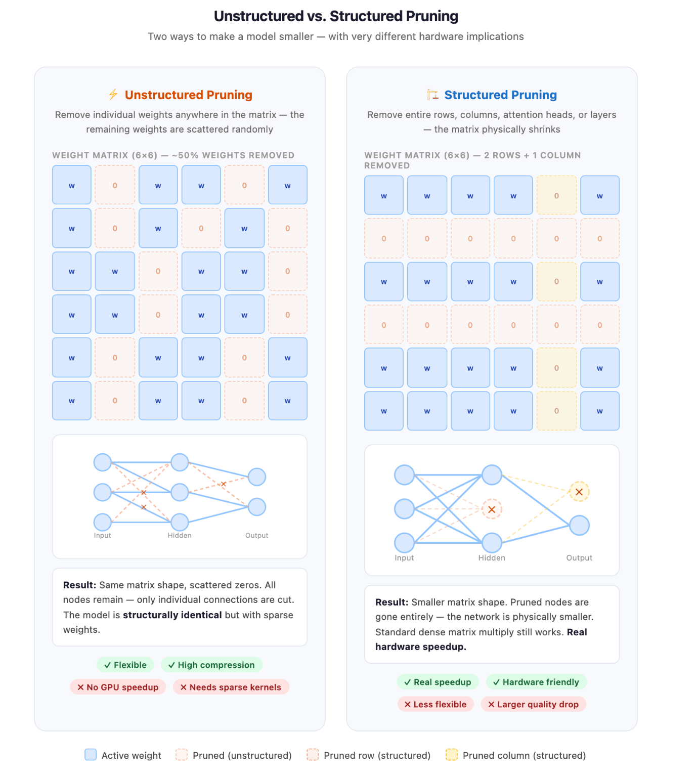
Unstructured vs. Structured Pruning
There are two fundamentally different ways to prune a model, and the distinction matters enormously in practice.
Unstructured pruning zeroes out individual weights anywhere in the network, regardless of their position. You might remove 50% of all weights, but the survivors are scattered randomly across the weight matrices. The matrices still have the same shape; they’re just sparse. This achieves excellent compression ratios and preserves quality well, but the resulting sparsity is irregular.
Modern GPUs are optimized for dense matrix multiplication, and they don’t get faster just because half the values are zero. Without specialized sparse kernels, unstructured pruning gives you smaller model files but not faster inference.
Structured pruning removes entire structural units such as full attention heads, complete neurons, and whole layers. The resulting model is smaller in shape, not just in values. Dense matrix multiplication still works, standard hardware still applies, and you get real throughput gains. The tradeoff is that structured pruning is less flexible: you’re forced to remove things in chunks, which can hurt quality more than removing the same number of individual weights in the most optimal positions.
The practical rule: if you need faster inference, use structured pruning. If you need a smaller model file and can tolerate sparse compute, unstructured pruning gives better quality-compression tradeoffs.
Magnitude Pruning
The simplest pruning method, and often a surprisingly competitive one: remove weights with the smallest absolute values. The logic is intuitive — a weight of 0.0003 multiplied against any reasonable input is going to produce an output close to zero. It’s not contributing much. Remove it.
Magnitude pruning works best when done iteratively: prune a small fraction of weights, fine-tune briefly to let the model recover, prune again, fine-tune again. Repeating this cycle gradually pushes the model toward sparsity without large quality drops at any single step. One-shot pruning, removing 50% of weights all at once, tends to hurt quality significantly because the model has no chance to redistribute the work done by removed weights.
The main weakness of magnitude pruning is that weight magnitude is a proxy for importance, not a direct measure of it. A small weight connected to a highly active neuron might matter more than a large weight in a dormant pathway. More sophisticated methods account for this.
Attention Head Pruning
Transformers use multi-head attention to let the model attend to different aspects of the input simultaneously. In theory, each head captures a different relationship. In practice, research consistently finds that many heads in a trained transformer are redundant, some heads attend to nearly identical patterns, and some barely activate on any input.
Studies on BERT and GPT-family models have shown that 30–40% of attention heads can often be removed with less than 1–2% degradation on downstream tasks. In some layers, you can remove nearly all heads and lose almost nothing.
The challenge is figuring out which heads to prune. Two common approaches:
Gradient-based importance scoring runs the model on a calibration dataset and computes how much each head’s output affects the final loss via its gradient. Heads with near-zero gradients aren’t influencing predictions and are safe to remove.
Taylor expansion scoring estimates the change in loss caused by zeroing out each head’s contribution, using a first-order Taylor approximation. It’s more principled than pure magnitude but computationally similar in practice.
After identifying low-importance heads, they’re masked out (set to zero) and the model is fine-tuned briefly so remaining heads can absorb the lost capacity. In practice, pruning 25–30% of attention heads in LLaMA-family models causes minimal quality loss while meaningfully reducing the compute cost of attention, which scales quadratically with sequence length.
Layer Dropping and Depth Pruning
The most aggressive form of structured pruning removes entire transformer layers. A 32-layer model becomes a 24-layer model. Every layer you drop eliminates its attention block, its MLP block, and all associated parameters, a clean, hardware-friendly reduction.
The key question is which layers to drop. A useful signal is the cosine similarity between a layer’s input and output: if a layer’s output is nearly identical to its input, the layer isn’t transforming the representation much, and it’s close to an identity function and can be removed with low impact.
ShortGPT, a 2024 paper, formalized this into a metric called Block Influence (BI) and showed that applying it to models like LLaMA-2 70B, you could remove 25% of layers with less than 2% degradation on most benchmarks. The layers most likely to be redundant are typically in the middle of the network — early layers build foundational representations, late layers refine outputs, but middle layers often contain significant redundancy.
Layer dropping is also used dynamically at inference time, a technique called early exit, where the model stops processing at an intermediate layer when its confidence is already high. Easy inputs skip the later layers entirely; only hard inputs use the full network. This can dramatically improve average-case latency without changing the model’s maximum capability.
SparseGPT and Wanda
Both GPTQ (from quantization) and magnitude pruning require either retraining or layer-wise optimization. For large models, even a brief fine-tuning run is expensive. SparseGPT and Wanda are one-shot pruning methods designed specifically for LLMs — no retraining required.
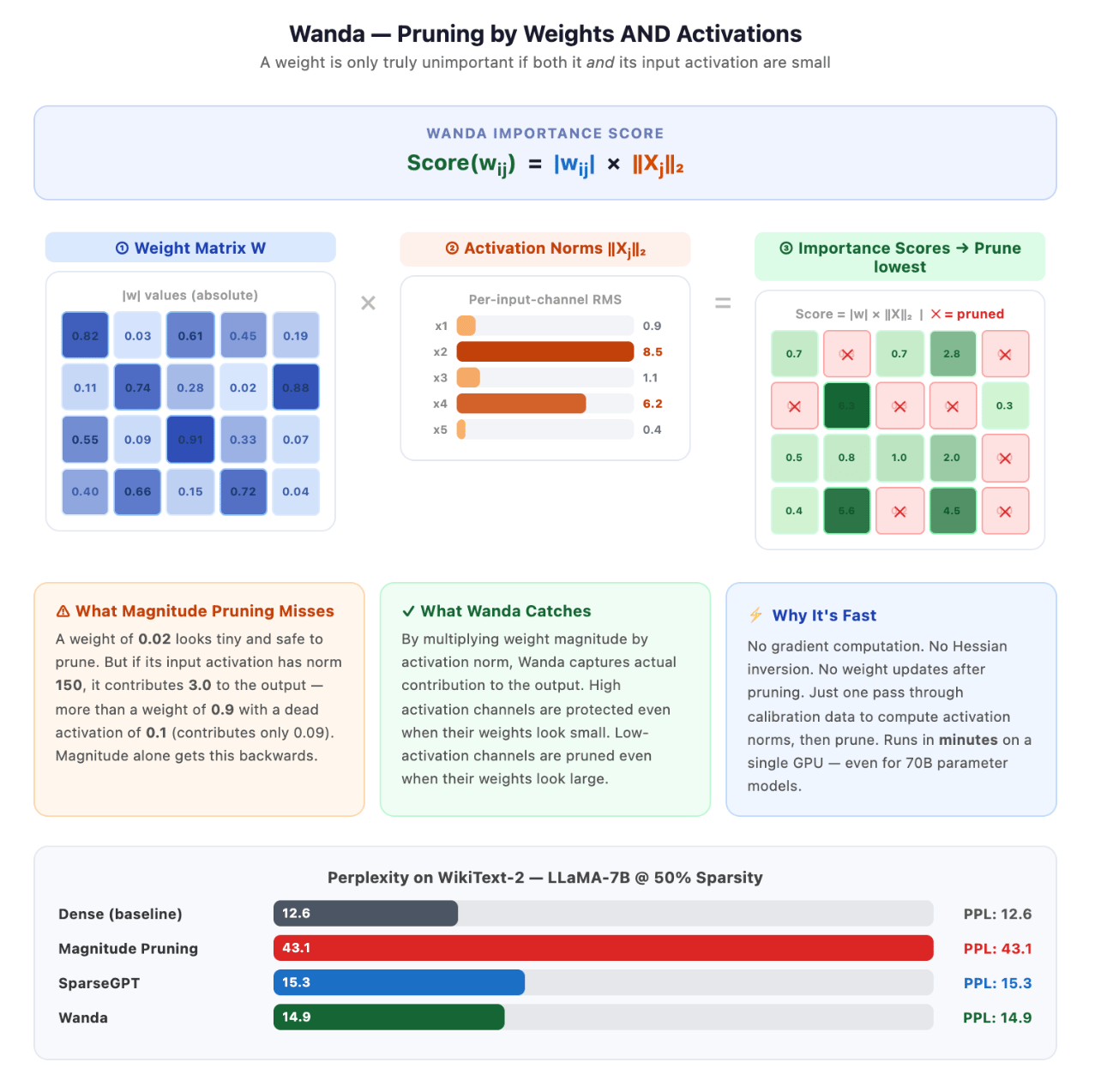
SparseGPT adapts the same second-order Hessian framework as GPTQ, but for pruning instead of quantization. When a weight is pruned, SparseGPT computes a correction to the remaining weights in the same layer to compensate for the lost contribution, minimizing changes to the layer’s output. This lets it prune 50% of weights from a 175B parameter model in a few GPU-hours, with perplexity increases of less than 1 point on WikiText-2. It also supports combined pruning + quantization in a single pass.
Wanda (Pruning by Weights and Activations) takes an even simpler approach. Instead of second-order corrections, it scores each weight by multiplying its magnitude by the RMS of its corresponding input activation:
importance(w_ij) = |w_ij| × ||x_j||₂
Weights with low scores, small magnitude, and low activation are pruned. This captures something magnitude pruning misses: a weight is only unimportant if both it and its input are small. A small weight connected to a large activation is still doing real work. Wanda runs in minutes, requires no gradient computation, and often matches or beats SparseGPT at 50% sparsity despite being far simpler.
To understand it in a simpler way, Wanda, unlike traditional pruning methods that take care of the weight, Wanda also considers how strongly neurons are activated during inference. The main intuition is that if a neuron is getting activated, then that weight is still important.
Hence, Wanda combines weight magnitude and activation importance to decide which weights to remove.
| Feature | Wanda | SparseGPT |
|---|---|---|
| Uses activations | Yes | Yes |
| Uses Hessian approximation | No | Yes |
| Speed | Very fast | Slower |
| Complexity | Simple | Advanced |
| Retraining needed | No | No |
| Accuracy retention | Very good | Better |
| Scalability | Excellent | Excellent |
Wanda became widely used because it can prune huge models like Meta LLaMA and Mistral to 50% sparsity in minutes on a single GPU, and that too with minimal quality loss without retraining.
That is extremely valuable for:
- GPU cost reduction
- Edge deployment
- Faster inference
- Lower VRAM usage
Our next article will dive deeper into the specifics of these two methodologies.
The Hardware Reality
GPUs are designed for dense tensor operations. When half of a matrix is zeros, the GPU still processes the full matrix; it just multiplies a lot of values by zero very quickly. The memory savings are real (you can store sparse matrices more compactly), but the compute savings depend entirely on having sparse-aware kernels.
NVIDIA partially addressed this with 2:4 structured sparsity on Ampere and later architectures (A100, H100). The constraint is specific: for every group of 4 consecutive weights, exactly 2 must be zero. This regular sparsity pattern lets the hardware skip the zero multiplications efficiently. NVIDIA’s Sparse Tensor Core implementation achieves close to 2x speedup on sparse operations — but only if the sparsity pattern satisfies the 2:4 constraint exactly. Unstructured sparsity gets none of this benefit.
For CPU inference, things work better because libraries like llama.cpp can make better use of sparse models. CPUs are often limited by how fast they can load data from memory, so skipping zero weights means less data needs to be loaded, which can improve performance.
FAQ’s
Do I need to retrain my model after quantization?
No, usually you do not need retraining. Techniques like GPTQ, AWQ, and LLM.int8() can quantize a pretrained model directly using a small sample dataset. Retraining is mainly needed when using extremely low precision, like INT3, or for tasks that require very high accuracy.
What’s the difference between GPTQ and AWQ — which should I use?
Both are popular quantization methods used to make LLMs smaller and faster.
- GPTQ focuses on reducing model size while keeping accuracy as close as possible to the original model. It works layer by layer and is widely supported in many tools.
- AWQ (Activation-aware Weight Quantization) pays more attention to important activations in the model, which often helps preserve quality better, especially for chat and instruction-following models.
In simple terms:
- Use GPTQ if you want broad compatibility and good compression.
- Use AWQ if you care more about maintaining response quality and are running inference on modern GPUs.
Can I apply both pruning and quantization to the same model?
Yes. In fact, many optimized LLM pipelines use both together.
- Pruning removes less important weights from the model.
- Quantization reduces the precision of the remaining weights.
Think of it like:
- Pruning = removing unnecessary parts
- Quantization = shrinking what is left
Combining them can reduce memory usage and improve inference speed even more.
Will users notice a difference with a quantized or pruned model?
Usually, not much, especially with moderate optimization.
For example:
- INT8 quantization often looks almost identical to the original model.
- 4-bit quantization may show small quality drops in complex reasoning tasks.
- Heavy pruning can sometimes make responses less accurate or more repetitive.
Most users will not notice changes for everyday tasks like chatting, summarization, or coding assistance unless the optimization is very aggressive.
How do I know which layers are safe to prune?
You usually do not manually pick layers at random. Modern pruning methods analyze:
- Weight importance
- Activation patterns
- Sensitivity of each layer
In general:
- Attention and feed-forward layers often contain many removable weights.
- Early and final layers are usually more sensitive and should be pruned carefully.
Tools like SparseGPT and Wanda automatically decide which weights are less important.
Conclusion: The First Half
LLM inference is not just one simple technique but includes a stack of techniques, and Part 1 of the article covered the first two techniques. Both quantization and pruning are important techniques for optimization. Some of that excess is numerical — weights stored at a precision they never needed. Some of it is structural — heads, layers, and connections that contribute marginally to outputs. Both forms of excess are recoverable without significantly sacrificing the model’s intelligence, and modern methods like AWQ, GPTQ, Wanda, and SparseGPT make that recovery fast, practical, and increasingly automatic.
A 70B parameter model that would have required eight A100s to run in FP16 can now be quantized to INT4, pruned of its most redundant structure, and served from a two-GPU setup, with most users unable to tell the difference.
But quantization and pruning only take you so far. They work at the model level — on the weights themselves. The other half of the inference optimization story plays out at the generation level: how tokens are produced, how memory is managed during a forward pass, and how the inherently sequential nature of autoregressive decoding can be subverted.
That’s where Part 2 picks up.
In the next article, we’ll cover Knowledge Distillation, training a small model to think like a large one, the technique that produced Phi, Mistral, and most of the efficient model families you’re likely already using. Then, KV Caching, the memory management engine that makes serving long-context conversations at scale even possible, includes PagedAttention, grouped-query attention, and prefix reuse. And finally Speculative Decoding, the cleverest trick in the stack, where a small draft model guesses ahead so the large model can verify multiple tokens in parallel, fundamentally changing the economics of latency-sensitive inference.
The model you optimize in Part 1 is the model you serve in Part 2. Together, these techniques form the complete picture of how modern AI systems actually run.
Thanks for learning with the DigitalOcean Community. Check out our offerings for compute, storage, networking, and managed databases.
About the author
With a strong background in data science and over six years of experience, I am passionate about creating in-depth content on technologies. Currently focused on AI, machine learning, and GPU computing, working on topics ranging from deep learning frameworks to optimizing GPU-based workloads.
Still looking for an answer?
This textbox defaults to using Markdown to format your answer.
You can type !ref in this text area to quickly search our full set of tutorials, documentation & marketplace offerings and insert the link!
 This work is licensed under a Creative Commons Attribution-NonCommercial- ShareAlike 4.0 International License.
Become a contributor for community
Get paid to write technical tutorials and select a tech-focused charity to receive a matching donation.

DigitalOcean Documentation
Full documentation for every DigitalOcean product.

Resources for startups and AI-native businesses
The Wave has everything you need to know about building a business, from raising funding to marketing your product.
The developer cloud
Scale up as you grow — whether you're running one virtual machine or ten thousand.

Start building today
From GPU-powered inference and Kubernetes to managed databases and storage, get everything you need to build, scale, and deploy intelligent applications.
